The Growing Neural Gas and Merge Growing Neural Gas Algorithms
Growing Neural Gas (NGN) is a topology preserving (see this blog for a demonstration) or this explaination) extension to the `Neural gas (NG) <>`__ approach is usefull for learning when an underlying topology is not known (as in the case of the `Self-organizing maps (SOM) <>`__ algorithm). When it comes to time series data (such as trajectories), an extension to the neural gas algorithm has been approached (Merge Neural Gas (MNG)) and a combination with the GNG leads to the Merge growing neural gas (MNGN) approach. It adds a context memory to the neurons of the NGN and is useful for recognising temporal sequences and with a single weighting parameter, can be reduced to a regular NGN for which an implementation is available.
This notebook allows experimenting with the (M)NGN algorithms on our own vanilla numpy implementation (which can be executed on the GPU with Cupy). The package uses modern python tools such as poetry, attrs (a focus has been laid on those two for this release), and sphinx and mypy/pylint/black for documentation and coding standards.
At first, let us import the necessary modules and set up loggin (aka. boilerplate code)
from neurovision.mgng.mgng import MergedGNG, lemniscate, get_dymmy_2D_data, repr_ndarray
import matplotlib.pyplot as plt

import ipywidgets as widgets
from ipywidgets import interactive, Layout

import numpy as np

import logging

logging.basicConfig(level=logging.ERROR,
                    format='%(name)s {%(filename)s:%(funcName)s:%(lineno)d} %(levelname)s - %(message)s',
#                     format='%(name)s [%(asctime)s] {%(filename)s:%(funcName)s:%(lineno)d} %(levelname)s - %(message)s',
#                     format='{%(filename)s:%(funcName)s:%(lineno)d} %(levelname)s - %(message)s',
                    datefmt='%m-%d %H:%M')

logger = logging.getLogger("jupyter")
logger.debug("test")

%matplotlib inline
def show_topology(mgng: MergedGNG):
    for n, row in enumerate(mgng._connections):
            ind = np.nonzero(row)
            # print(ind)
            for i in ind[0]:
                plt.plot([mgng._weights[i,0], mgng._weights[n,0]], [mgng._weights[i, 1],mgng._weights[n,1]], '-y')
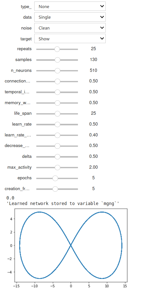
Interactive playground
Use the following cell to interactively test on a data set (parameterized and rotated Bernoulli lemniscate):
mgng = None

logging.getLogger('neurovision.mgng.mgng').setLevel(logging.WARNING)

def learn(type_, data, noise, target, repeats,samples,
      n_neurons, connection_decay,
      temporal_influence,
      memory_weight,
      life_span,
      learn_rate,learn_rate_neighbors,
      decrease_activity,
      delta, max_activity, epochs, creation_frequency):

    std = 0.0 if noise == 'Clean' else 1.0
    print(std)

    if data=='Single':
        X =  np.hstack(
            [lemniscate(0, x, samples) for x in np.random.randn(repeats)*std + 10]
        )
    else:
        X = get_dymmy_2D_data(repeats, std, samples)

    global mgng

    if type_ == 'MGNG':
        mgng = MergedGNG(
            n_neurons=n_neurons,
            n_dim=2,
            connection_decay=connection_decay,
            temporal_influence=temporal_influence,
            memory_weight=memory_weight,
            life_span=life_span,
            learn_rate=learn_rate,
            learn_rate_neighbors=learn_rate_neighbors,
            decrease_activity=decrease_activity,
            delta=delta,
            max_activity=max_activity,
            debug=False,
            creation_frequency=creation_frequency

        )

        mgng.learn(X.T,1)
        Y,Z = mgng.get_active_weights()
        plt.plot(Y.T[0, :], Y.T[1, :], '*g')
        plt.plot(Z.T[0, :], Z.T[1, :], '*r')

        for x,y in zip(mgng._weights, mgng._context):
            plt.plot([x[0],y[0]],[x[1],y[1]],'-k')
        show_topology(mgng)

    if target=='Show':
        plt.plot(X[0, :], X[1, :])
    display("Learned network stored to variable `mgng`")


interactive_plot = interactive(
    learn,
    type_=['None','MGNG','GNG'],
    data = ['Single','Double'],
    noise = ['Clean', 'Noisy'],
    target = ['Show','Hide'],
    repeats=(1,50),
    samples=(10,250,10),
    n_neurons=(20,1000),
    connection_decay=(0.0,1.0),
    temporal_influence=(0.0,1.0),
    memory_weight=(0.0,1.0),
    life_span=(0,50),
    learn_rate=(0.0,1.0),
    learn_rate_neighbors=(0.0,0.8),
    decrease_activity=(0.0,1.0,0.01),
    delta=(0.0,1.0),
    max_activity=(1.0,3.0),
    epochs=(1,10),
    creation_frequency=(1,10)
)
# output = interactive_plot.children[-1]
# output.layout.height = '350px'
display(interactive_plot)